The title is inspired by article, Imperial Paste - Infantry tactic in mind of Emperor (written in Chinese).
In book Imperial Bayonets, I found this phase:
The second assumption is that people are capable of marching like machines with an absolutely standardized pace. In the short term this is not true, but long term, with a eye to the statistical mean of all normally distributed events, the marching will distill down to an average probably very close to the regulated cadence and length of pace.
In reality, long term marching “distill” down to average exactly, but not because of “long term” itself. Obviously, if the amount of moving is independent increments, $X_i \sim N(\mu, \sigma^2)$, thus the distribution of the “total moving”, the sum of those random variables, is:
This distribution will not converge to the mean $N\mu$, but diverge. In other word, if all of men moved “independently”, the result will look like this:
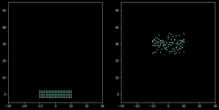
The result seems not what we want. It’s obvious that moving of units don’t follow a such random pattern, they observing around to do subtle moving to maintain the formation. This seems to imply multi-agent methodology, see MAgent repo for a cool gif example.
Setting some basic rules, expecting some interesting pattern emerging is a interesting enough, but maybe too complex to this problem. Can we use a “reduced form” model to denote the process, not bothering those complex generative or “structure form” model?
A probabilistic graph model(PGM) or energy based model are easy to build. For example, we can set “ideal” position and define a energy (loss) for deviating from that “ideal” setting. See wiki for a detailed description.
PGM and energy based model are not easy to inference, which usually require costly sampling technique. We instead resort to Gaussian Process, a relatively effective method compared to general PGM. See wiki for a detailed description.
Assume units move only in y-axis. There’s a “ideal”(expected) positions for every unit each timestamp. For example, assume a uniform linear motion, $y_i(t)=y_i(0)+\mu t$, where $\mu$ is expected speed.
We will model deviating from ideal position, the error term:
Where $oy_i(t)$ means observed y-position unit $i$ at time $t$. $y_i$ is ideal value. $ey_i(t)$ is a zero mean random variable. The joint distribution of $ey_i(t)$ is given by:
Where $K(F, F)$ is kernel matrix, given by:
Where $F_1,F_2$ are features of unit $i,j$ at a time, which are defined by $(X_i,Y_i,T_i)$. Thus two unit $i,j$ are different even they differ only in time $T$. Here the form of $k$ is derived from Squared Exponential kernel form. $w$ is weight vector.
Intuitively, we want two error terms which close in ideal position and time will tend to have same deviating tendency. Time is a natural requirement, otherwise, for example, a unit at $t=5.00000$ and $t=5.00001$ may have opposite direction:
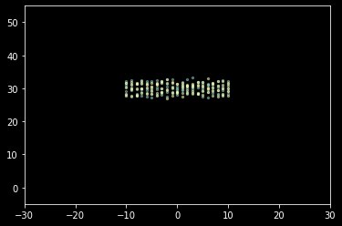
Location requirement is easy to understand. We may expect at same time unit which are close to each other will have consistent deviating tendency, leading a smoother placement instead of a zigzag shape. In other hand, closing to each other at different timestamp having same tendency may imply a “unseen” terrain obstacle, which slow units passing it temporarily.
Take 30 frames to display (enlarging deviating for illustration):
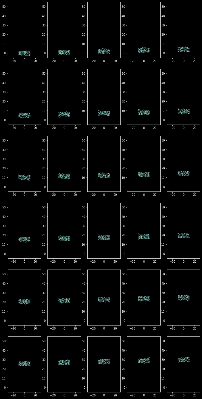
Animating figure(gif):
Well, it’s more like a Yankee parading rather than “imperial” maneuvering…